
Paperspace Deployments are containers-as-a-service that allow you to run container images and serve machine learning models using a high-performance, low-latency service with a RESTful API.
In this tutorial, you learn how to start deploying a model to an endpoint using Gradient.
Gradient Deployments lets us perform effortless model serving to an API endpoint.
During this tutorial we learn how to use Gradient to deploy a machine learning model using a high-performance, low-latency microservice with a RESTful API.
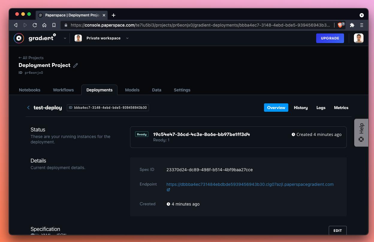
Gradient Deployments let you deploy a container image to an API endpoint for hosting or inference.
In Part 1 of this tutorial, we’re going to deploy a generic version of Streamlit to an endpoint. This is an extremely quick exercise to demonstrate how quickly we can serve a container to an endpoint in Gradient.
In Part 2, we’re going to increase complexity and serve an inference endpoint. We first train a model with Gradient Workflows and then deploy it.
Let’s get started!
In Part 1 of this tutorial, our goal is to deploy an application as fast as possible. Once we get a handle on the look and feel of a Deployment, we then move on to Part 2 during which we train and deploy an inference server capable of responding to a query.
I this first part, we’re going to use the Streamlit demo application that is available as a starter Deployment within the Gradient console.
Here is what we’re going to do:
Let’s create our new project!
If we haven’t already created a project in the Gradient console, we need to do that first. We’re going to select Create a Project from the homepage of our workspace. Alternatively, if we already have a project that we’d like to use, we can select that project as well. We can create as many projects as we like no matter what service tier we’re on – so feel free to create a new project to keep things nice and tidy.
If we haven’t made a Project yet in Gradient, create a new one now. Here we’ve named our new project Deployments Tutorial. We add more than one Deployment to this project as we progress through his tutorial.
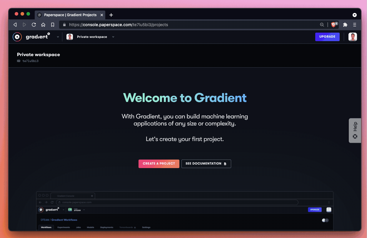
Great! We should now have a new project in Gradient with the name Deployments Tutorial.
After we create a new project, we’re going to create a new Deployment within that project.
Let’s go ahead and create a Deployment within our project. Once we’re within the project in the UI (we can confirm this by seeing the name of our project in the top left along with the button to navigate back to All Projects) let’s tab over to the Deployments panel and click Create.
Let’s name our new Deployment Streamlit Deployment and then click Deploy. This generates a deployment using the pre-made deployment spec and options provided by Paperspace.
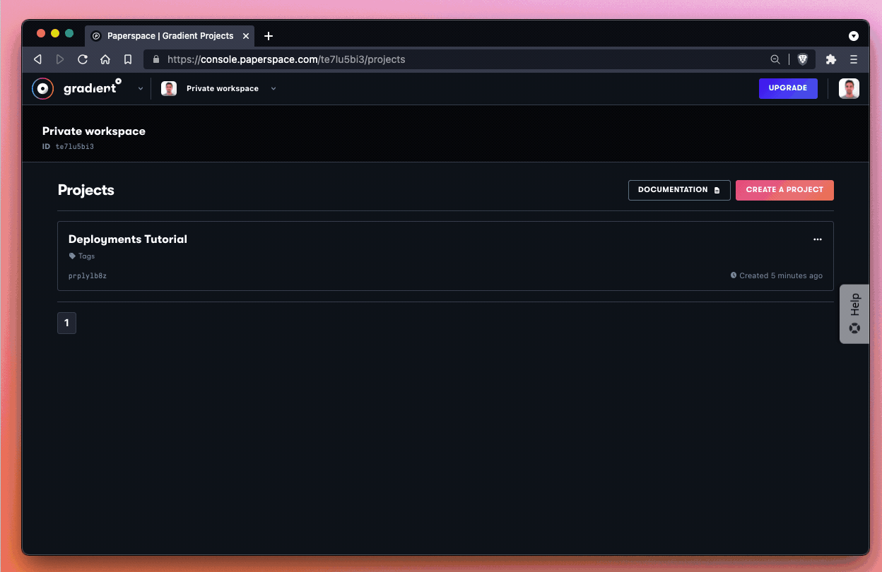
Excellent! While our Deployment is spinning-up, let’s take a look at the Deployment spec that we ran:
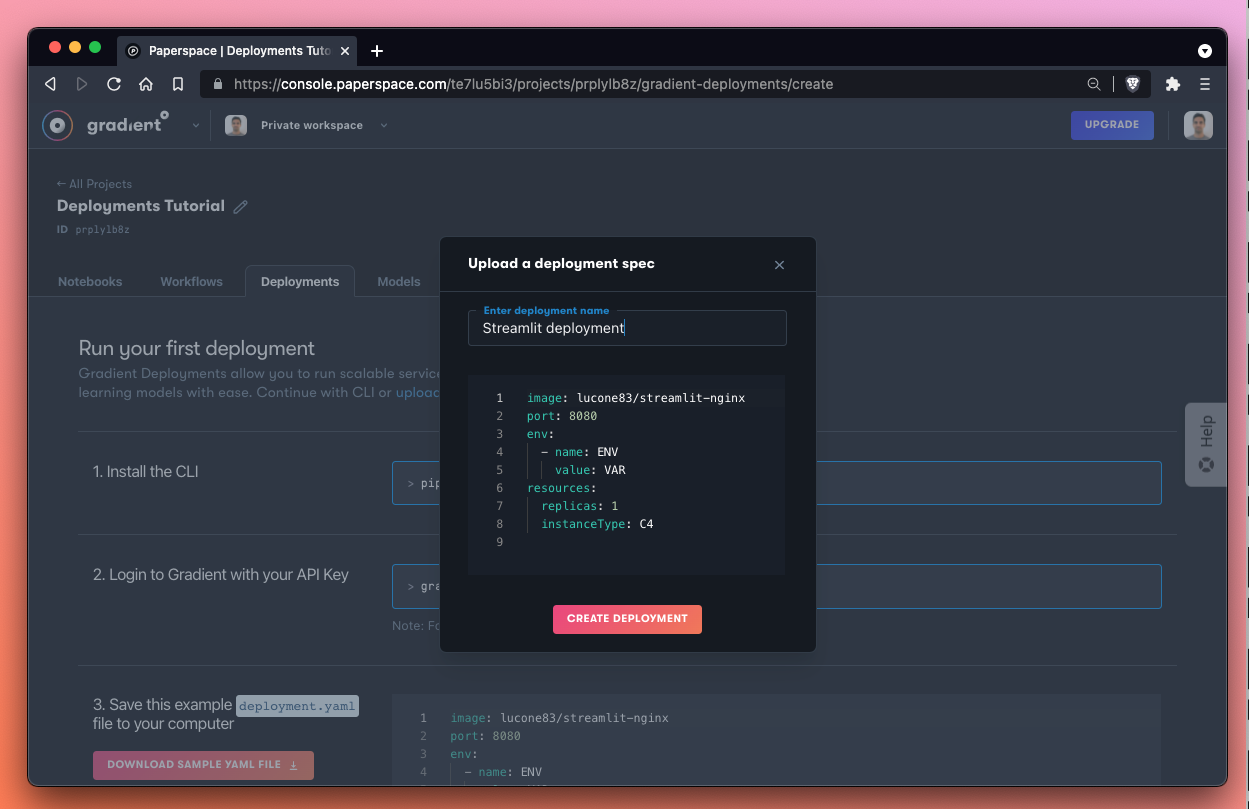
The spec for this Deployment looks like this:
image: lucone83/streamlit-nginx
port: 8080
env:
  - name: ENV
    value: VAR
resources:
  replicas: 1
  instanceType: C4
Let’s break down our instructions to Gradient:
image - the specified image or container for Gradient to pull from DockerHubport - the communication endpoint that the Deployment server should expose to the open internetenv - environment variables to apply at runtimeresources - compute instance to apply to this jobAs we can see, there is a good amount of configuration options available. If we wanted to change the instance type, for example, we would need to modify the resources block. If we wanted to upgrade our processor to a C5 instance, for example, we would write:
resources:
  replicas: 1
  instanceType: C5
That’s all there is to it! For more information on the Deployment spec, be sure to read the docs.
Meanwhile, let’s see the result of our Deployment:
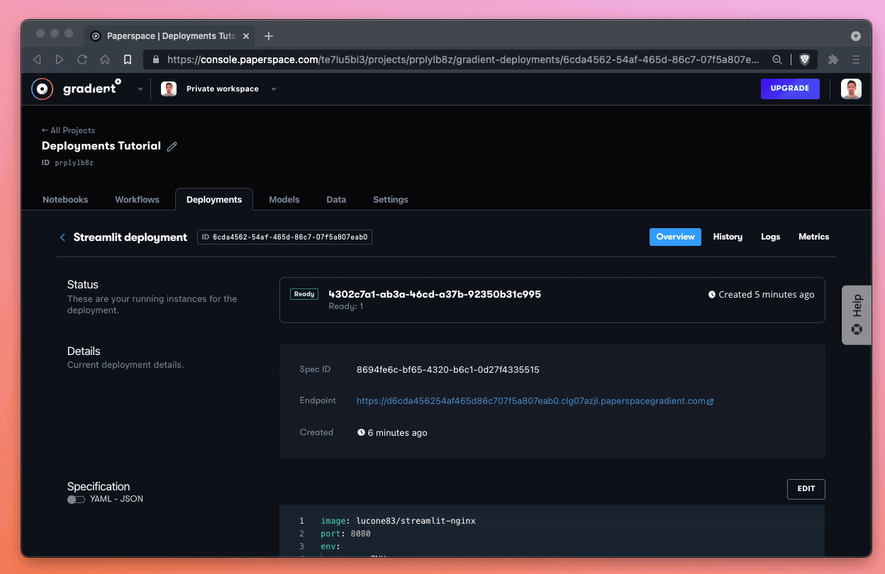
Excellent! It takes about 30 seconds for our Deployment to come up, but once it does the UI state changes to Ready and the link to our Streamlit Deployment brings us to a hosted endpoint where we can demo a number of Streamlit features.
We’ve now successfully launched our first Deployment!
In the next part of the tutorial we take a look at doing a more end-to-end Gradient Deployments project where we train a model first and then host it to an endpoint.
In Part 2 of this tutorial, we are going to upload an ONNX model to Gradient and serve it to an endpoint as a Deployment. By the end of this section we can query the endpoint to run inference.
For Part 2 of this tutorial, we are going to reference the sample ONNX model GitHub repository which contains the sample ONNX model as well as a sample Deployment spec.
To deploy a model endpoint, we first need to upload the model to Gradient. After that, we reference the model in our Deployment spec which allows us to serve the model as an endpoint.
The first thing we do is grab the model files from the demo repo and upload them as a model object in the Gradient user interface.
These are the model files we are looking to upload to Gradient:
/models/fashion-mnist/fashion-mnist.onnx
/models/fashion-mnist/fashion-mnist.py
The model files we need to download and then upload to Gradient are available in the models/fashion-mnist directory of the onnx-deployment repo, are also available via the GitHub UI.
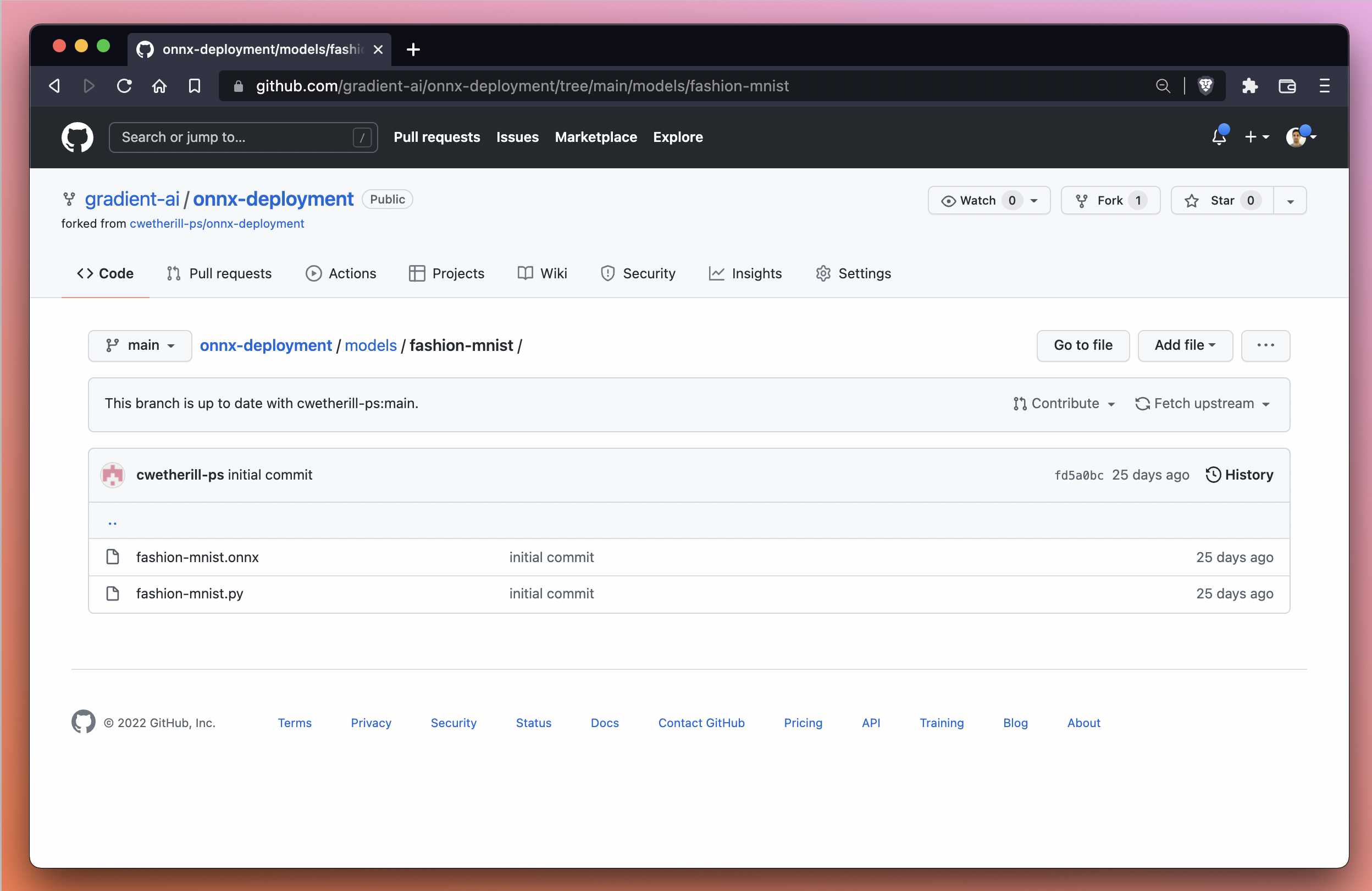
We first need to download the files to our local machine before we can upload to Gradient. We can accomplish this from our local machine via the command line or via the GitHub user interface.
In the command line we can first cd into our local directory of choice. Here we use /downloads:
cd ~/downloads
Then we can use the git clone command to clone the repo to our local machine:
git clone https://github.com/gradient-ai/onnx-deployment.git
We can then open the repo that we downloaded and navigate to onnx-deployment/models/fashion-mnist to find our files.
Alternatively, if we prefer to use the GitHub UI, we can use the download button and then unzip the repo to the preferred destination on our local machine. The download button is located under the Code pull-down in the GitHub UI, as seen below:
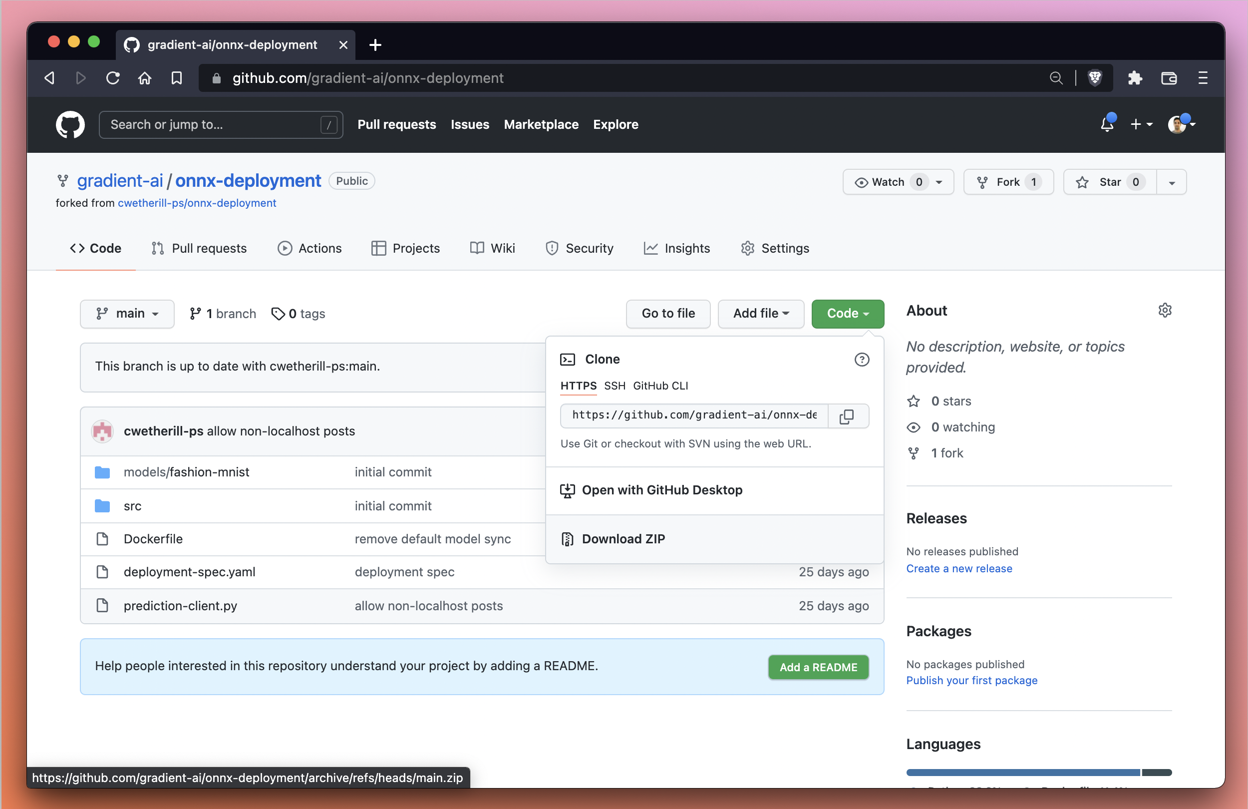
Next, we’re going to upload the model files to Gradient as a model object.
To upload a model to Gradient, we first hop over to the Models tab within the Gradient console.
From here, we select Upload a model which brings up a modal that allows us to select or drag-and-drop files to upload as a model.
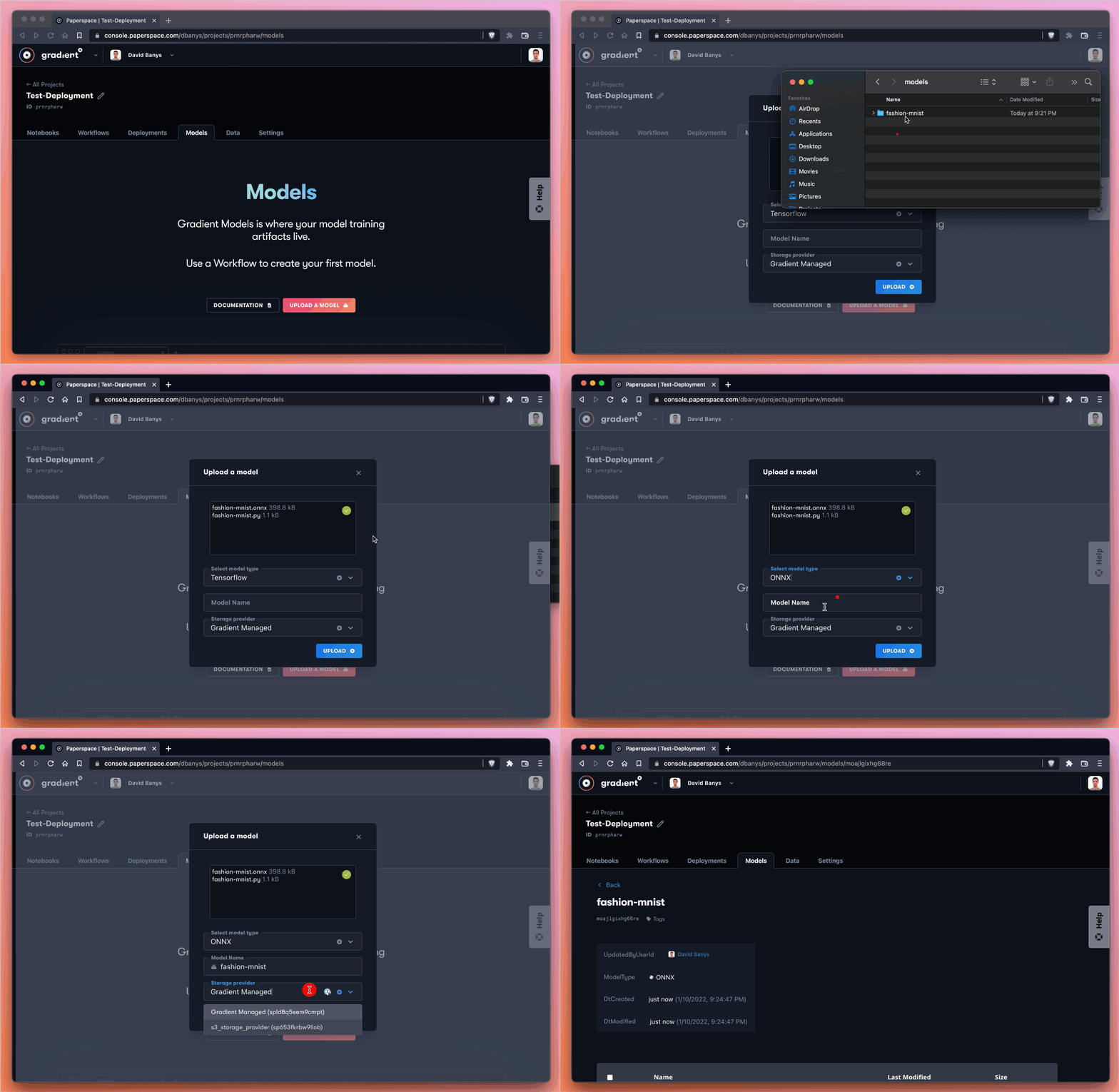
These are the steps we take in the Upload a model modal:
fashion-mnist.onnx and fashion-mnist.py) from our local machineSelect model type and select ONNXStorage providerBy selecting Gradient Managed, we are telling Gradient that we’d like to use the native storage and file system on Gradient rather than setting up our own storage system.
All we have to do now is click Upload and wait for the model to be available, which should take a few moments.
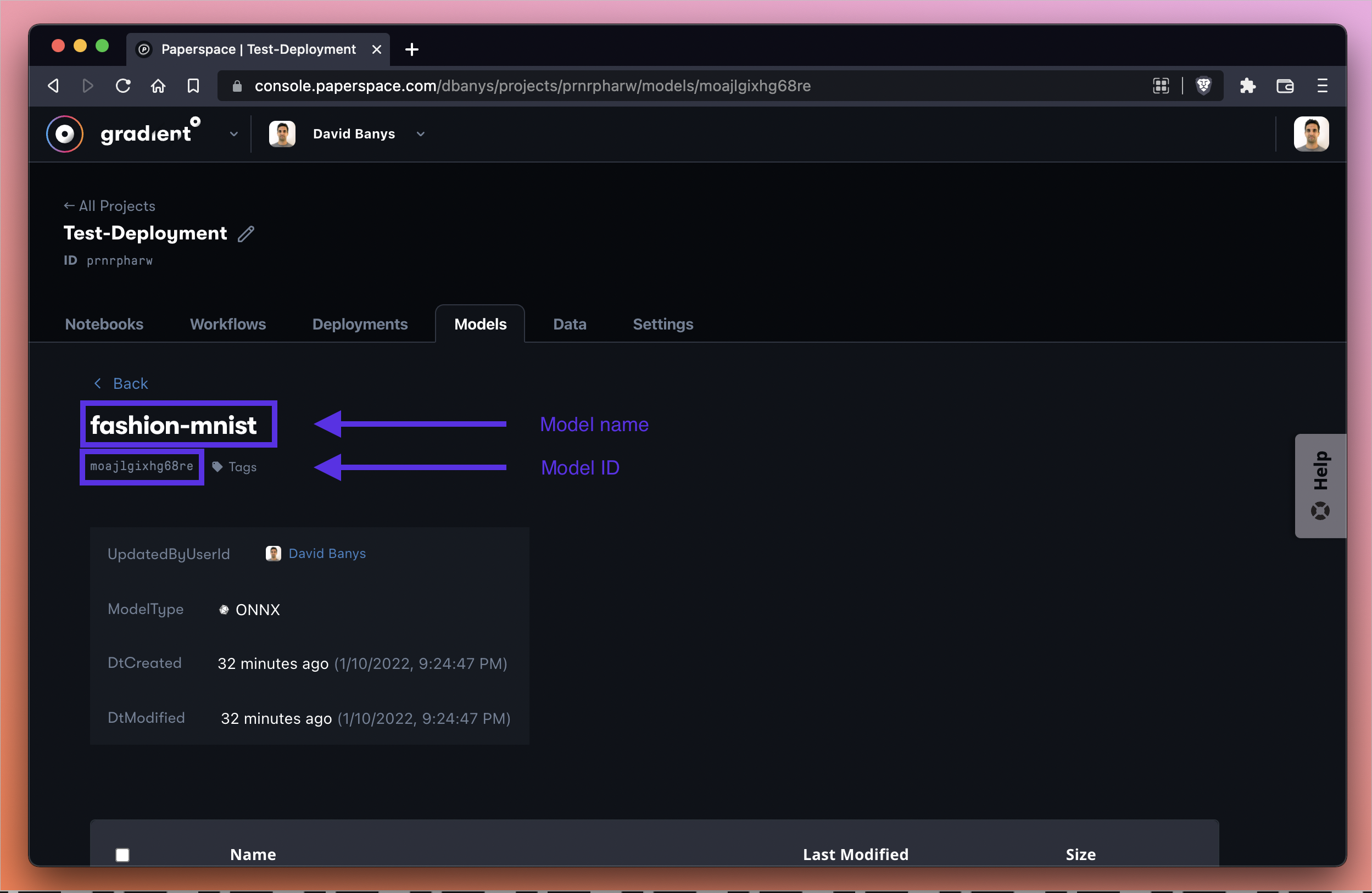
At this point we should see that our model has both a name (in our case fashion-mnist) and a model ID (in our case moajlgixhg68re). Your own model name depends on the name you give your model, and the ID depends on the computer-generated ID that Gradient assigns you.
In any case, we need to reference these two pieces of information in the next step, so let’s be sure to hold on to them!
Now we’re going to create another Deployment within the same project we used in Part 1 (which we titled Deployments Tutorial).
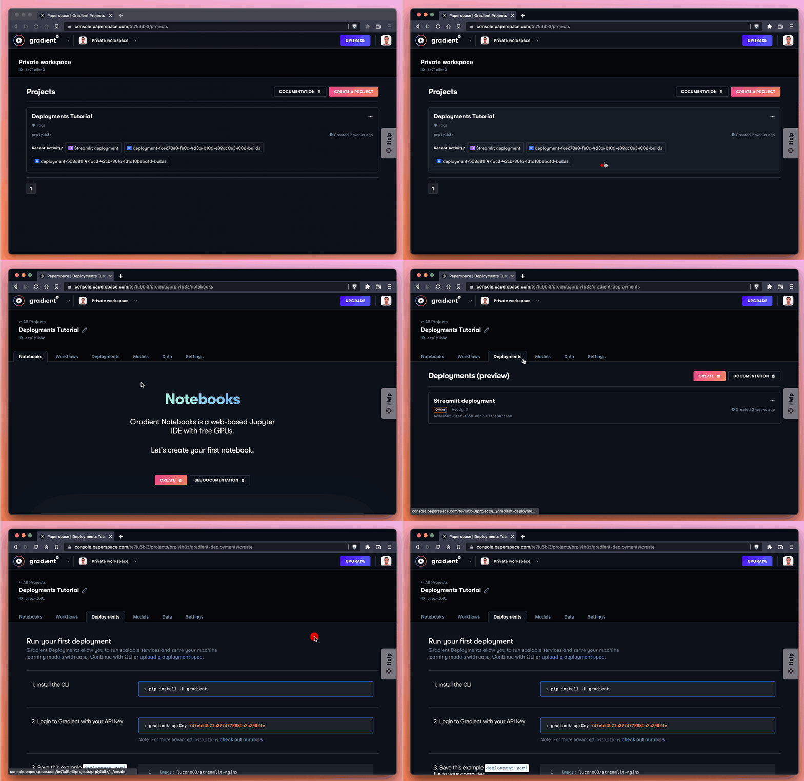
From the Deployments tab of the Gradient console, we first select Create.
Next, we use the Upload a Deployment spec text link to bring up the YAML spec editor.
By default, the spec looks like this:
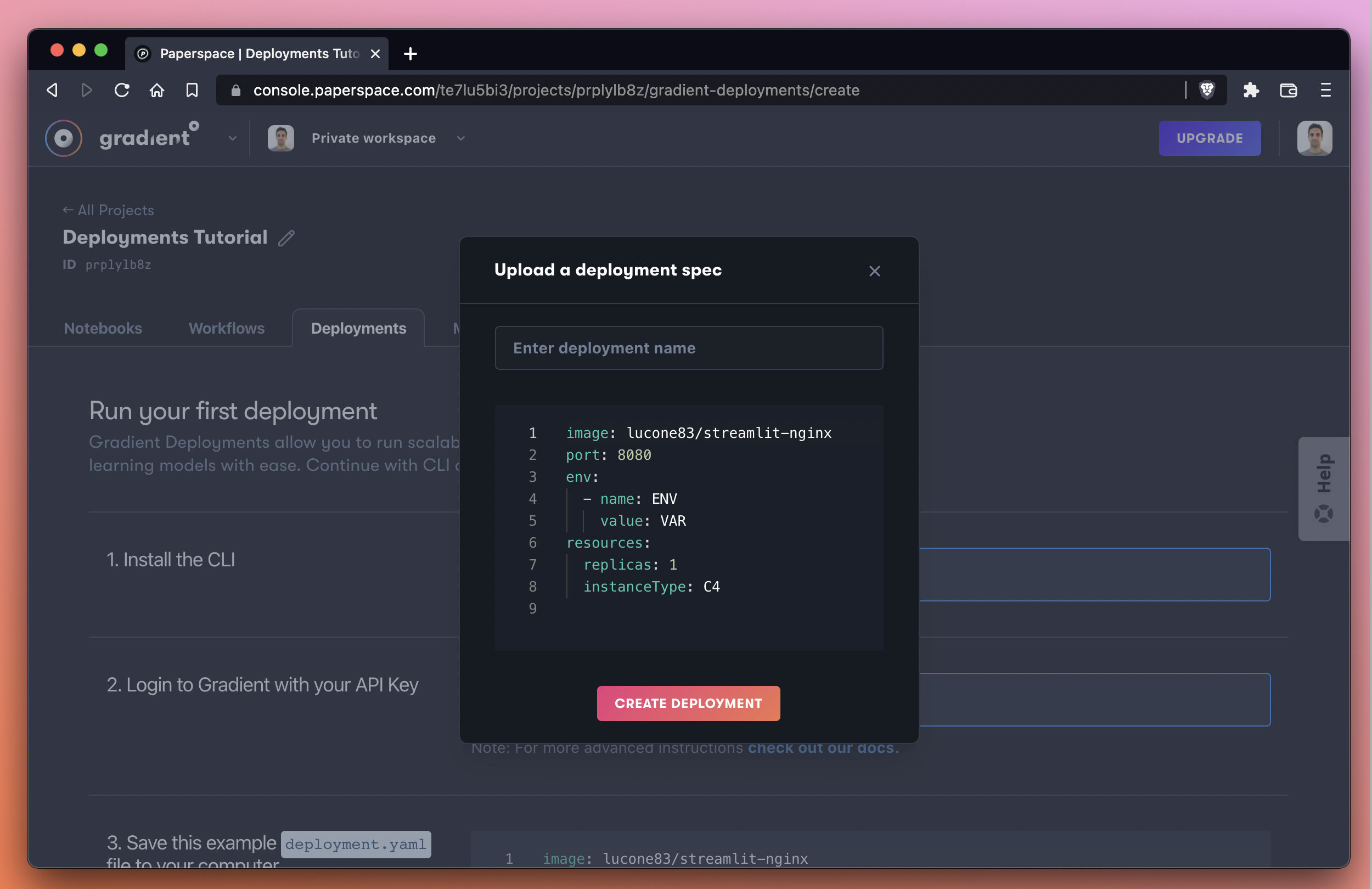
Instead of the default spec, we’re going to overwrite the spec with our own spec as follows:
image: cwetherill/paperspace-onnx-sample
port: 8501
resources:
  replicas: 1
  instanceType: C4
models:
  - id: moajlgixhg68re
    path: /opt/models/fashion-mnist
Here is an explanation of the Deployment spec:
image - the Docker image or container that we want Gradient to pullport - the port number we would like to open to the public web to make requestsresources - the machine we are specifying to run our Deployment – in this case a single instance (also known as a replica) of a C4 machine (see available machines here)models - the id and path of the model we would like to deployAfter a few minutes we should see that our instance is now running:
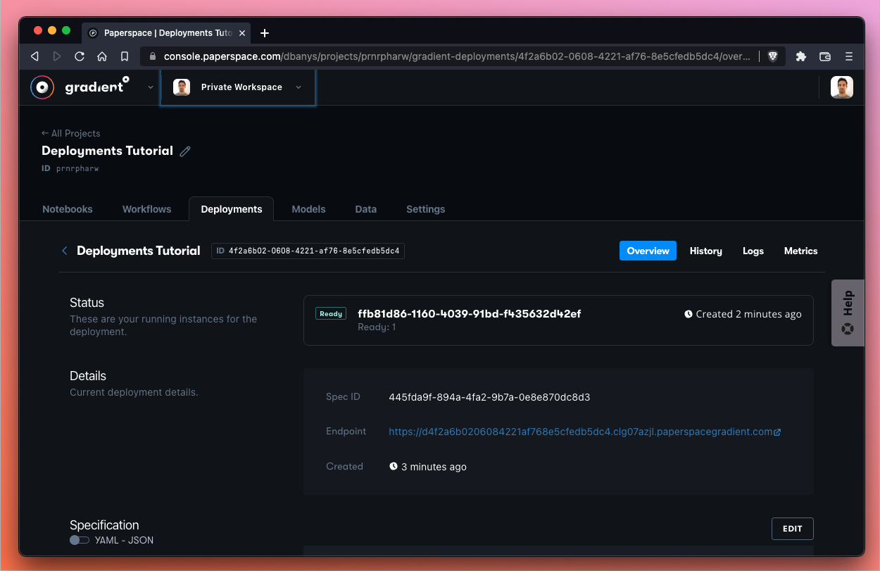
Nice! We now have a Deployment that is up and running.
To verify that this runtime is up and running, we can use a nifty helper endpoint that the Paperspace team included with the runtime, which is available at <endpoint>/healthcheck.
The <endpoint> parameter is available in the Details section of the Deployment. Here is a close-up of the details pane:

Here’s what it looks like when we try the endpoint. We are going to use our endpoint and append /healthcheck to the URL since we know that this container has defined such a method.
Every Deployment generates a unique endpoint URL – for this reason we purposely do not provide the URL of the endpoint from this tutorial and instead ask the user to create a new Deployment to obtain a unique Deployment endpoint.
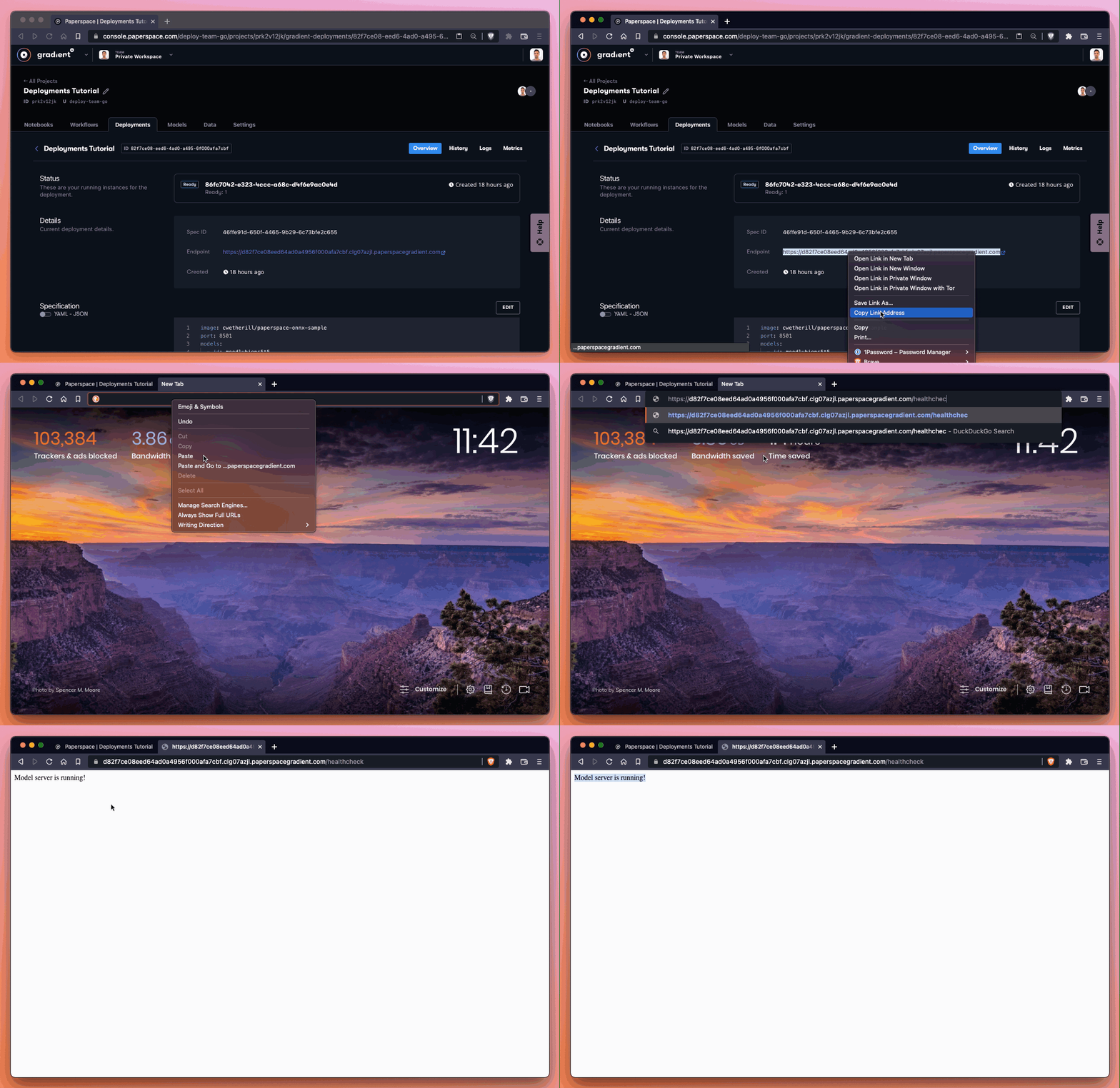
Our model server is running – excellent!
We can also cURL this endpoint from the command line on our local machine to achieve the same result. Here is what that command looks like:
curl https://d4f2a6b0206084221af768e5cfedb5dc4.clg07azjl.paperspacegradient.com/healthcheck
Let’s also try another method which has been made available to us in this demo repository by the Paperspace team. This method tells us about our metadata and we can find it at <endpoint>/v1/models/fashion-mnist/metadata.
We should see that this URL also produces a response – in this case the method allows us to inspect the request/response formats provided by the endpoint.
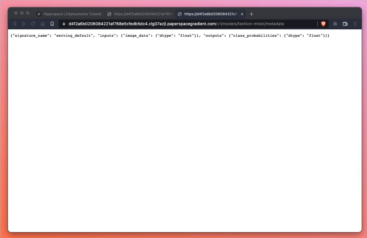
If we’re using cURL in the terminal our command line entry would look like this:
curl https://d4f2a6b0206084221af768e5cfedb5dc4.clg07azjl.paperspacegradient.com/v1/models/fashion-mnist/metadata
Great! We’ve now successfully deployed the model that we uploaded previously and we’ve confirmed with two separate helper methods that the model server is running and that the endpoint request/response formatting is as follows:
{
   "signature_name":"serving_default",
   "inputs":{
      "image_data":{
         "dtype":"float"
      }
   },
   "outputs":{
      "class_probabilities":{
         "dtype":"float"
      }
   }
}
Next we’re going to query the endpoint in a notebook.
Let’s go ahead and hit the endpoint now that we’ve successfully deployed our model. We do so with a Gradient Notebook which allows us to view the image we are submitting to the endpoint via matplotlib.
First, we create a new notebook using the TensorFlow 2 template.
To create the notebook, return to the Gradient console. Ensuring we are in the same project (Deployments Tutorial in our case) as our Deployment, we then go to the Notebooks tab in the Gradient console and select Create.
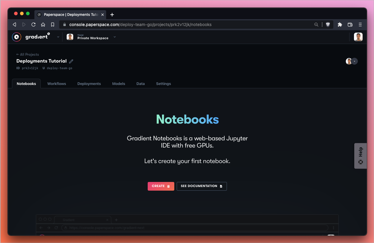
Let’s select the TensorFlow 2 runtime (currently Tensorflow 2.6.0) to use when querying our endpoint.
Next, let’s select a machine. Since we are running inference on the endpoint (and not in the notebook itself) we can run the lightest CPU-based machine available. Let’s select the Free CPU instance if it’s available. If the free instance is not available due to capacity, we can select the most basic paid CPU instance available.
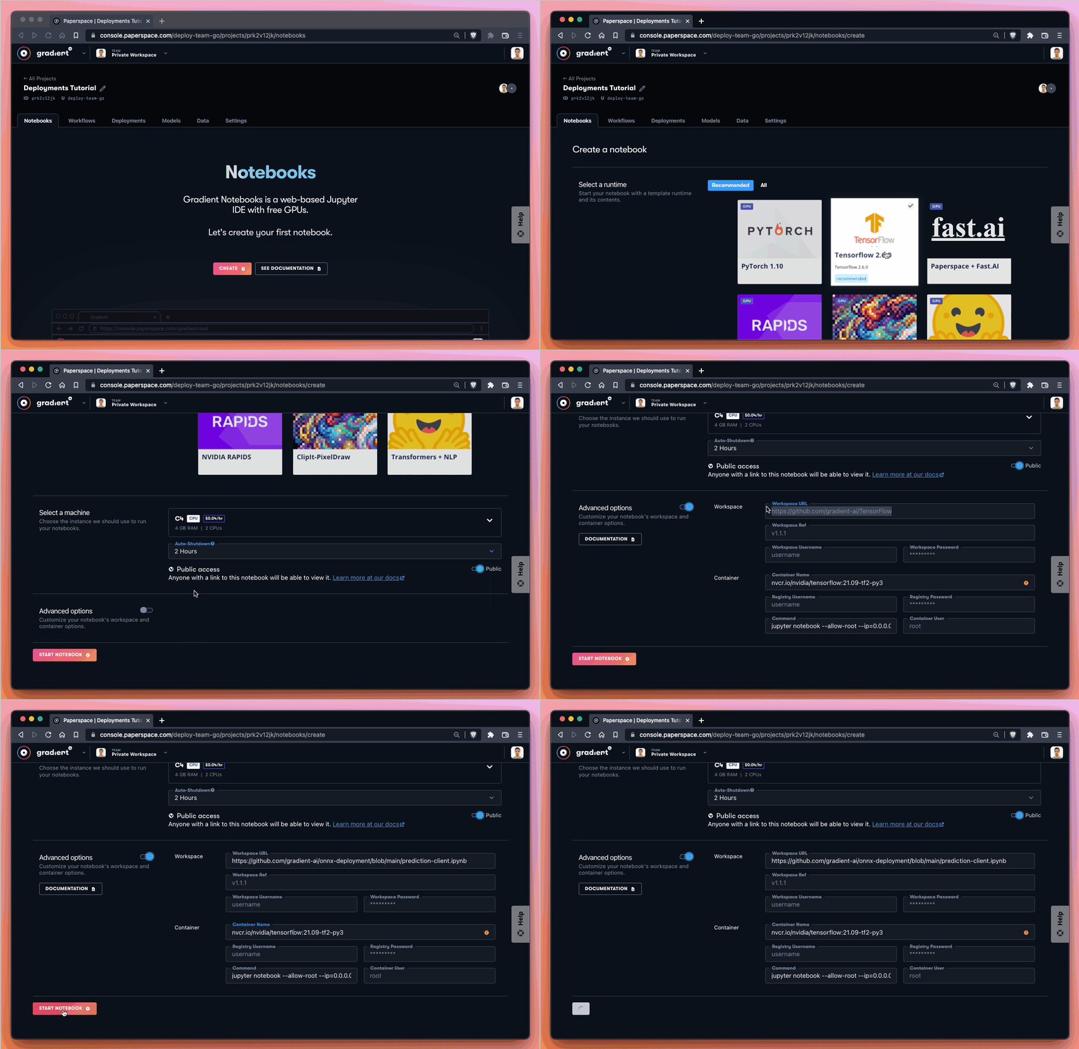
We now take advantage of Advanced options when we create our notebook to tell Gradient to pull the notebook file that is located in the GitHub repo.
The link to the file which we use as the Workspace URL in Advanced options is as follows:
https://github.com/gradient-ai/onnx-deployment/blob/main/prediction-client.ipynb
After that we click Start Notebook and wait for our notebook to spin-up!
When our notebook spins up, we should see something like this:
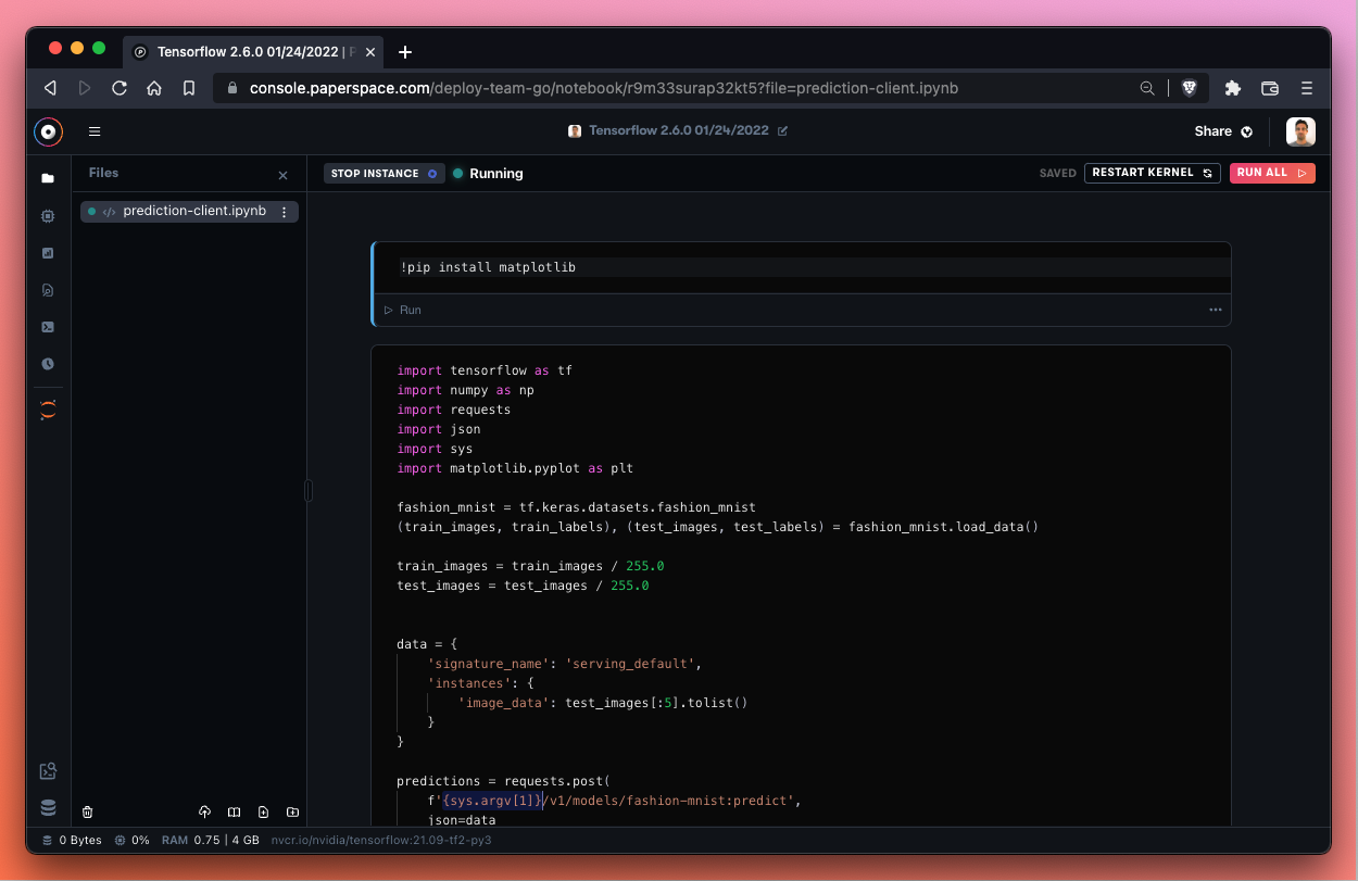
Let’s go ahead and run the first cell which installs matplotlib.
Next, we need to input our Deployment endpoint as a replacement for the {sys.argv[1]} variable. If we need to get our Deployment URL once again, we can visit the Gradient console, then Deployments, then click on the Deployment and copy the Endpoint parameter under Details.
When we have our Deployment endpoint, we drop it in as a replacement for the {sys.argv[1]} variable.
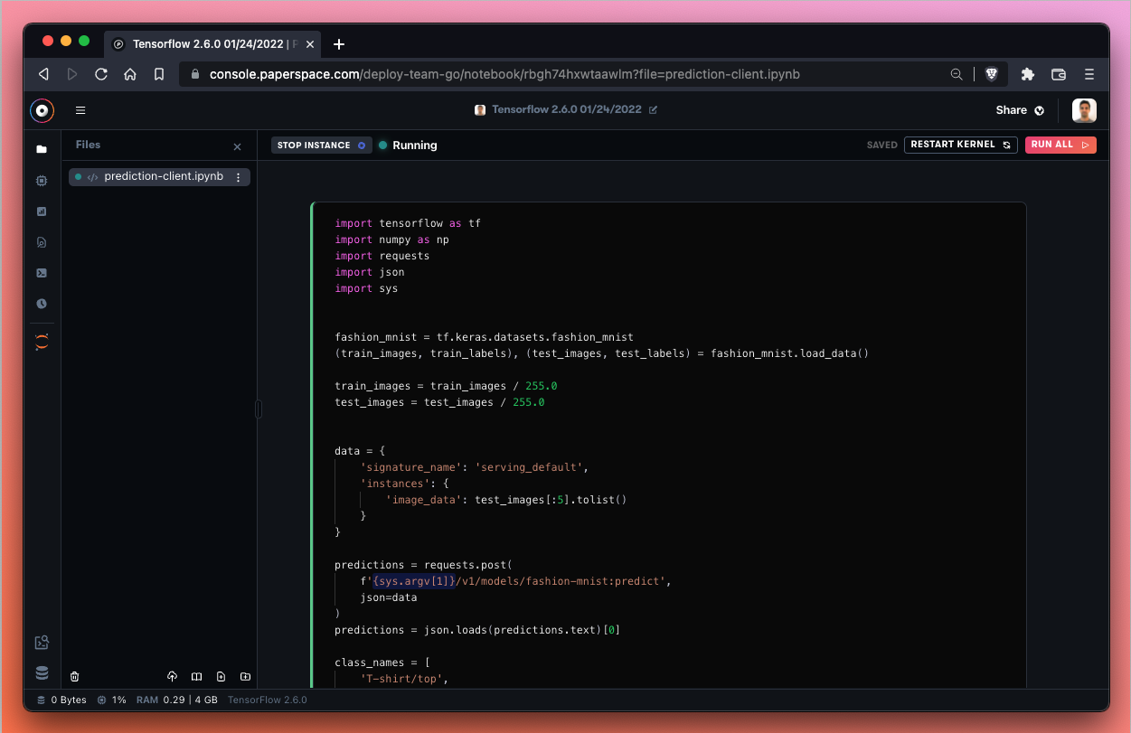
Now we can run the notebook!
After we paste our unique Deployment endpoint into the notebook prediction request parameter, we can run the cell. We should then be able to generate a prediction.
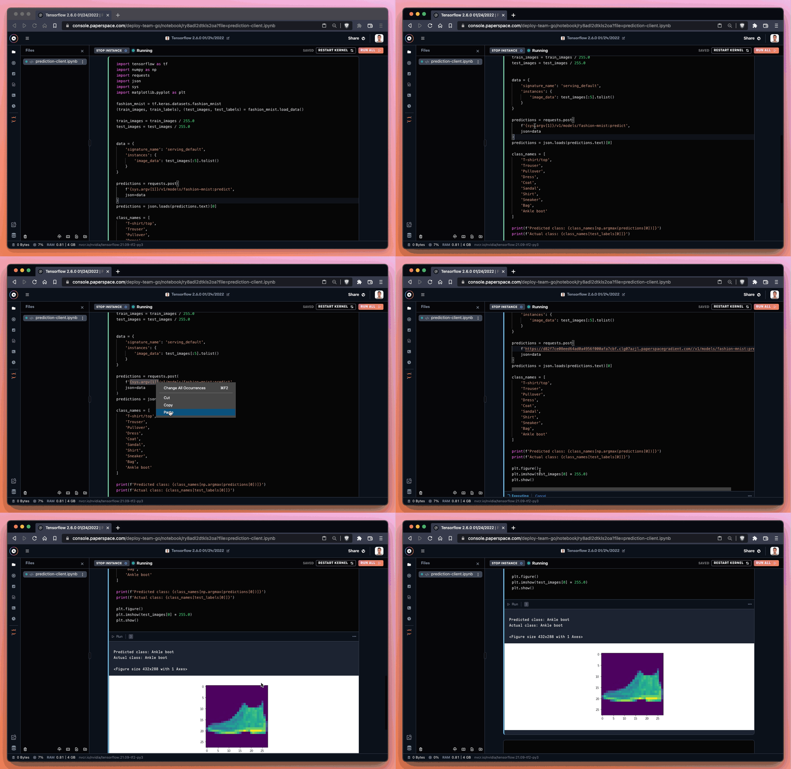
If everything works correctly, we should be able to generate a prediction. In our case, we correctly identified the image as an Ankle boot!
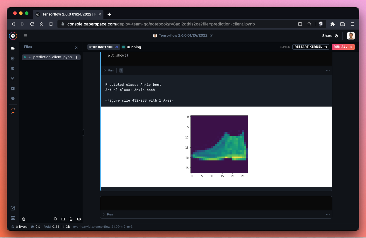
Success! Nice job identifying that ankle boot! We ran inference from an endpoint and returned the prediction to a notebook – awesome!
In Part 2 of this tutorial, we’ve accomplished the following:
cURL requests in the terminal.ipynb file from the demo repository and make requests to the endpointOnce a model is deployed to an endpoint with Gradient Deployments the possibilities are truly unlimited.
In Part 2 of this tutorial we used a notebook to query the endpoint so that we could visualize the image submitted to the endpoint with matplotlib. We could hit the endpoint from the command line of our local machine or from within an application we are writing.
We can also use Gradient Workflows to make a request to the endpoint, or we could use third party tools like Postman to make requests.
In short, there are a lot of possibilities. Whatever we decide to do next, the important thing is to go step by step and make sure each piece of the Deployment is working as you progress.
If you have any questions or need a hand getting something to work – please let us know! You can file a support ticket.